The Inspiration

My initial inspiration for plotting the progression of teams in the FA Cup by League, came from this graphic by FiveThirtyEight on the Champions League. I have mentioned it in other posts, but to re-iterate, I have found emulating other people’s graphics a great way to develop data visualisation skills. It not only gets you thinking about what makes the particular graphic so compelling, but also makes you wonder how it was created. I don’t know if the FiveThirtyEight graphic was built with R, but felt I could make an approximation of it for my own purposes whilst also adding my own personal mark to it. Andy Cotgreave gives a fantastic synopsis of this learning strategy in the latest (episode 14) Storytelling with Data Podcast:

If you want to improve your skills in this area or learn to visualize data, then my advice is to go and read Austin Kleon’s book Steal Like an Artist. It’s a really short book. It’s a great manifesto on how to become a great artist. But his principle is you learn by copying others, and when you copy people honorably, you take their style. And even in the process of copying it, you’re actually putting your own style into that. Or your understanding of what they did. And this is a great way of learning. Take a look at what other people do. Take inspiration and put those into your own work. Eventually, through that, you will discover your own voice and your own style that will evolve over time.

Scrappy Scraping

I’ve sourced the FA Cup results for the past 8 seasons from Wikipedia. Luckily, this data is readily available on Wikipedia, but on the downside there is not a consistent structure across the pages. So not only do I need to scrape and wrangle the data for one of the Wiki pages, I also need to assess and then amend as approriate based on differences in other pages.

To read and scrape the data, I will be using the rvest package by Hadley Wickham. I have only recently learnt how to web scrape, with very little previous knowledge of web languages, so it still feels like a bit of a dark art to me. But I’ll show the process, warts and all, in the hope someone might find it useful. Like always, I will be harnessing the power of the tidyverse to tame and tidy my data:

library(tidyverse)
library(rvest)

First up, I will get a vector of the URLs I want to scrape (i.e. the 8 URLs for each of the past 8 tournaments):

# Create vector of each season - e.g. 2010-11, 2011-12 etc
seasons <- paste(2010:2017, 11:18, sep = "-")

# Use vector above to create vector of urls for each wiki page
urls <- paste0("https://en.wikipedia.org/wiki/", seasons, "_FA_Cup")

urls

## [1] "https://en.wikipedia.org/wiki/2010-11_FA_Cup"
## [2] "https://en.wikipedia.org/wiki/2011-12_FA_Cup"
## [3] "https://en.wikipedia.org/wiki/2012-13_FA_Cup"
## [4] "https://en.wikipedia.org/wiki/2013-14_FA_Cup"
## [5] "https://en.wikipedia.org/wiki/2014-15_FA_Cup"
## [6] "https://en.wikipedia.org/wiki/2015-16_FA_Cup"
## [7] "https://en.wikipedia.org/wiki/2016-17_FA_Cup"
## [8] "https://en.wikipedia.org/wiki/2017-18_FA_Cup"

This vector of URLs will be used to iterate over the scraping function.

I will attempt to unravel this rather unwieldy function, by splitting it into a few parts. I won’t go into minute detail on each step, but will highlight elements of the code that I found particularly useful in helping me battle through the nuances of the wiki pages and reach the ultimate goal of a nice, clean dataset at the end.

The function will take just one input, the URL for the wikipedia page:

# scraping function
fa_cup_scrape <- function(url) {

  Sys.sleep(2)

# assign url
fa_source <- url

The first step is to extract the schedule of the FA cup in each season (how many games are played in each round?). This is needed as when I extract the games played in each round, there is nothing to identify which round it is. So I will want to attach the name of the round to each game.

Common functions of the rvest package are to read the HTML of the page (read_html), select the required node(s) (html_node, html_nodes) and then extract the text or table (html_text, html_table). A great intro to rvest can be found here. I am no authority on the mechanics of web-scraping and I have found it involves a lot of trial and error. I have had success in the past using a selector gadget to identify the CSS selector to use as the node. However, in this case I couldn’t quite get what I wanted. I eventually stumbled upon a Stack Overflow post where someone had used an xpath selector instead. The xpath below did the trick and it was just a case of changing the element as required. Once I have the required table in a dataframe, I filter to only keep the ‘proper’ rounds (i.e. ignore the qualifying rounds) and then take the number of fixtures for each round and uncount. This function, as you might expect, effectively does the opposite of a count. Taking the number of fixtures for each round and then creating the equivalent number of rows. Straight away there are discrepancies in the layout of the Wiki pages, so I need 3 slightly different methods depending on the season:

# Extract schedule table - how many ties in each round?
# use uncount() to create a row for every tie in each round
if (as.integer(str_sub(fa_source, -14, -11)) < 2013) {
  schedule <- read_html(fa_source) %>% 
  html_nodes(xpath = '//*[@id="mw-content-text"]/div/table[3]') %>% 
  html_table() %>% 
  .[[1]] %>% 
  filter(toupper(str_sub(Round, -6, -1)) == "PROPER" | str_sub(Round, 1, 4) == "Semi" | Round == "Final") %>% 
  select(Round, no_of_ties = `Number of fixtures`) %>% 
  uncount(no_of_ties)
} else if (as.integer(str_sub(fa_source, -14, -11)) < 2017) {
  schedule <- read_html(fa_source) %>% 
  html_nodes(xpath = '//*[@id="mw-content-text"]/div/table[2]') %>% 
  html_table() %>% 
  .[[1]] %>% 
  transmute(Round, no_of_ties = Clubsinvolved / 2) %>% 
  uncount(no_of_ties)
} else {
  schedule <- read_html(fa_source) %>% 
    html_nodes(xpath = '//*[@id="mw-content-text"]/div/table[2]') %>% 
    html_table() %>% 
    .[[1]] %>% 
    select(Round = X1, X6) %>% 
    filter(toupper(str_sub(Round, -6, -1)) == "PROPER" | str_sub(Round, 1, 4) == "Semi" | str_sub(Round, 1, 7) == "Quarter" | Round == "Final") %>% 
    transmute(Round , no_of_ties = as.integer(X6)) %>% 
    uncount(no_of_ties)
}

Now to extract the fixtures played in each round. The “.attendee” CSS selector extracts each team that played in each round from the ‘First Round Proper’ onwards, and the team name is also followed by the level of the club (i.e. their league) in parenthesis (this is super handy as I need to know this!). Unfortunately, the later rounds (Semi-Final and Final) are not always included within the “.attendee” nodes, but if not, they can be extracted from the “.faway” and “.fhome” nodes. I can then combine these into 1 vector of all teams that played from the 1st round through to the final. I split the teams into home and away teams and then stick together to get a row for each tie, with the home team and away team as the columns. There is then some fiddling about to remove the ties that were replays, as I only want to include each team once for each round.

# Extract teams
# number in brackets indicates level (level 1 = Premier league, level 2 = championship etc)
fa_cup_teams <- read_html(fa_source) %>% 
  html_nodes(".attendee") %>% 
  html_text() 

# doesn't include the final (and for some years the semi-final too), so scrape this too
final <- read_html(fa_source) %>% 
  html_nodes(".faway , .fhome") %>% 
  html_text() 

# create 1 vector of all teams from 1st round proper to final
fa_cup_teams <- c(fa_cup_teams, final)

home <- seq(1, length(fa_cup_teams), 2)
away <- seq(2, length(fa_cup_teams), 2)

# create table of ties - home team in 1st column, away team in 2nd column
all_ties <- tibble(home_team = fa_cup_teams[home],
               away_team = fa_cup_teams[away])

# exclude replays
unique_ties <- all_ties %>% 
  filter(!(lag(home_team) == away_team & lag(away_team) == home_team & row_number() != 1)) %>% 
  filter(!(lag(home_team) == home_team & lag(away_team) == away_team & row_number() != 1)) %>% 
  filter(!(lag(home_team) == "Droylsden (6)"  & away_team == "Droylsden (5)")) %>% 
  filter(!(lag(home_team) == away_team & lag(away_team) == home_team & row_number() != 1))

ties <- unique_ties %>% 
  add_column(round = schedule$Round)

I now have a simple dataset consisting of a row for each game played, with a column for home team, away team and the round. I will now put the home and away teams into the 1 column, filter out the rounds prior to the Third Round, convert the ‘level’ of the club into their League and convert the round description into a number (starting at 1 for the Third Round):

# put home and away teams into 1 column
# exclude rounds before 3rd round
teams <- select(ties, team = home_team, round) %>% 
  rbind(select(ties, team = away_team, round)) %>% 
  filter(!toupper(round) %in% c("FIRST ROUND PROPER", "SECOND ROUND PROPER")) %>% 
  mutate(level = as.integer(str_extract(team, "[0-9]")),
         league = case_when(level == 1 ~ "Premier League",
                            level == 2 ~ "Championship",
                            level == 3 ~ "League One",
                            level == 4 ~ "League Two",
                            TRUE ~ "Non-League"),
         round_number = case_when(toupper(round) == "THIRD ROUND PROPER" ~ 1,
                                  toupper(round) == "FOURTH ROUND PROPER" ~ 2,
                                  toupper(round) == "FIFTH ROUND PROPER" ~ 3,
                                  toupper(round) == "SIXTH ROUND PROPER" ~ 4,
                                  toupper(round) == "QUARTER-FINALS" ~ 4,
                                  toupper(round) == "SEMI-FINALS" ~ 5,
                                  round == "Final" ~ 6)) %>% 
  arrange(round_number, team) %>% 
  mutate(team = str_remove_all(team, " \\(.*\\)"))

# level missing for final team from 2016 on
if (as.integer(str_sub(fa_source, -14, -11)) >= 2016) {
  teams <- teams %>% 
    arrange(team, round_number) %>% 
    mutate(level = case_when(is.na(level) ~ lag(level),
                             TRUE ~ level),
           league = case_when(level == 1 ~ "Premier League",
                              level == 2 ~ "Championship",
                              level == 3 ~ "League One",
                              level == 4 ~ "League Two",
                              TRUE ~ "Non-League")) %>% 
    arrange(round_number, team)
    
}

#winner - 1 element vector of winner
winner <- read_html(fa_source) %>% 
  html_nodes(xpath = '//*[@id="mw-content-text"]/div/table[1]') %>% 
  html_table() %>% 
  .[[1]] %>% 
  filter(X1 == "Champions") %>% 
  pull(X2) %>% 
  str_remove_all(" \\(.*\\)")

# use the data on teams to get remaining data for winner
winner_league <- teams %>% 
  filter(team == winner) %>% 
  select(team, level, league) %>% 
  unique() %>% 
  mutate(round_number = 7)

# final dataset for each season
fa_cup_table <- teams %>% 
  select(-round) %>% 
  rbind(winner_league) %>% 
  mutate(season = str_sub(fa_source, -14, -8))

}

There is some final scraping and wrangling done above to make sure the data for The Final and Winner in each season is present and correct. Once that is done, I create my final dataset, fa_cup_table, ensuring the season being scraped is included in the data.

Finally, I have a function that will scrape for all seasons! After all this ugliness, the code to iterate the function to scrape each season is beautiful in its elegance and simplicity:

fa_cup_all <- map_df(urls, fa_cup_scrape)

The map_df function from the purrr package, takes a vector (in this case urls) and performs a function on each element in the vector, combining the final dataframe from each iteration (the fa_cup_table datasets) into 1 (fa_cup_all).

Why have I put you through this scraping torture? I guess the aim was to show that extracting data from the web is rarely clean and straightforward. This function was built up and amended as I worked through each season and discovered the nuances within. I was presented with many hurdles, and had to adapt the code and invent workarounds as required. The above is by no means the optimal solution to extracting the data I needed, but it is a solution, and it now allows me to visualise the data I have. Being able to extract data from the web is a powerful tool, enabling you to get access to all kinds of data that may interest you, and you can get started with with very limited knowledge of HTML, CSS etc.

Plot Preparation

Let’s take a look at the data:

head(fa_cup_all)

## # A tibble: 6 x 5
##   team             level league         round_number season 
##   <chr>            <int> <chr>                 <dbl> <chr>  
## 1 Arsenal              1 Premier League            1 2010-11
## 2 Aston Villa          1 Premier League            1 2010-11
## 3 Barnsley             2 Championship              1 2010-11
## 4 Birmingham City      1 Premier League            1 2010-11
## 5 Blackburn Rovers     1 Premier League            1 2010-11
## 6 Blackpool            1 Premier League            1 2010-11

tail(fa_cup_all)

## # A tibble: 6 x 5
##   team              level league         round_number season 
##   <chr>             <int> <chr>                 <dbl> <chr>  
## 1 Manchester United     1 Premier League            5 2017-18
## 2 Southampton           1 Premier League            5 2017-18
## 3 Tottenham Hotspur     1 Premier League            5 2017-18
## 4 Chelsea               1 Premier League            6 2017-18
## 5 Manchester United     1 Premier League            6 2017-18
## 6 Chelsea               1 Premier League            7 2017-18

For each team, in each season, I want to extract the furthest stage they reached in the competition (max_round). I’m then creating a new variable pos (position) based on the row number of the record once I have arranged the data by season, descending league and max_round. This is to solve a pretty niche plotting problem I encountered. In my plot I want to facet by season, whilst also retaining the order of the teams in each season by League and the furthest round they reached. This seemingly simple requirement was tripping me up, but thankfully I discovered this perfect blog post from Simon Jackson that solved the problem. Thanks Simon! Essentially, mapping this newly created pos variable as an aesthetic in the plot, instead of the team variable, enables the plot to order the data as requested (note later in the plot that scales = "free" in the facet_wrap is also needed).

# data prep ready for plot
fa_cup_plot <- fa_cup_all %>% 
  group_by(season, team, league) %>% 
  summarise(max_round = max(round_number)) %>% 
  ungroup() %>% 
  mutate(team = factor(team, levels = unique(team)),
         league = factor(league, levels = c("Premier League",
                                            "Championship",
                                            "League One",
                                            "League Two",
                                            "Non-League")),
         season = factor(season, levels = rev(unique(fa_cup_all$season)))) %>% 
  arrange(season, desc(league), max_round) %>% 
  mutate(pos = row_number()) 

I’m creating the colour palette based on the logos for each league because I like a carefully curated colour palette:

# colour palette
league_pal <- c("#3D1A5B", "#BD9941", "#808485", "#BB312F", "black")

I’m creating 2 supplementary datasets that will be used to add annotations to the final plot. I’m manually placing the annotations where I want them based on the aesthetics that will be used in the plot (I found that I had to recreate the factor levels for the season variable to enable the faceting in the final plot to remain as intended):

# labels and commentary for plot
size_labels <- tibble(pos = c(54, 32, 54), max_round = c(0.2, 0.2, 6.5), 
                      season = rep("2017-18", 3), label = c("20 teams", "24", "64\nteams")) %>% 
  mutate(season = factor(season, levels = rev(unique(fa_cup_all$season))))

commentary <- tibble(pos = c(28, 89, 218, 285), 
                     max_round = c(2.8, 3.1, 3.2, 3.2), 
                     season = c("2017-18", "2016-17", "2014-15", "2013-14"), 
                     label = c("No C'ship team has reached\nQ-F in last 2 seasons",
                               "Lincoln become first Non-League\nteam to reach Q-F since 1914",
                               "Reading last C'ship\nteam to reach S-F",
                               "League 1 Sheffield Utd\nreach S-F")) %>% 
  mutate(season = factor(season, levels = rev(unique(fa_cup_all$season))))

The Plot

I won’t focus too much on the code behind the plot, as I have covered highly customised ggplot2 graphs in other posts, and it feels like this blog post has already gone into extra-time and penalties:

# plot
# needed to plot geom_col twice for some reason as wanted it on top of lines but
# if i remove first geom_col it doesnt work - strange
# had to fiddle with geom_segment and y labels to get them where i wanted
ggplot(fa_cup_plot, aes(x = pos, y = max_round)) +
  geom_col(aes(fill = league), width = 1, show.legend = TRUE) +
  geom_segment(aes(x = -Inf, xend = Inf, y = 1, yend = 1), colour = "white", size = 0.01, alpha = 0.5) +
  geom_segment(aes(x = -Inf, xend = Inf, y = 2, yend = 2), colour = "white", size = 0.01, alpha = 0.5) +
  geom_segment(aes(x = -Inf, xend = Inf, y = 3, yend = 3), colour = "white", size = 0.01, alpha = 0.5) +
  geom_segment(aes(x = -Inf, xend = Inf, y = 4, yend = 4), colour = "white", size = 0.01, alpha = 0.5) +
  geom_segment(aes(x = -Inf, xend = Inf, y = 5, yend = 5), colour = "white", size = 0.01, alpha = 0.5) +
  geom_segment(aes(x = -Inf, xend = Inf, y = 6, yend = 6), colour = "white", size = 0.01, alpha = 0.5) +
  geom_col(aes(fill = league), width = 1, show.legend = FALSE) +
  geom_text(data = size_labels, aes(label = label), colour = "white", 
            hjust = if_else(size_labels$label == "64\nteams", 0.5, 0), size = 3.5, show.legend = FALSE, family = "DINAlternate-Bold") +
  geom_label(data = commentary, aes(label = label), 
             colour = "black", fill = "ivory", label.size = 0,
             hjust = 0, vjust = 0, size = 3.8, show.legend = FALSE, family = "DINAlternate-Bold") +
  geom_curve(data = commentary, aes(x = c(31, 89, 228, 285), xend = c(41, 69, 235, 277), 
                                    y = c(2.8, 5.4, 4.5, 4.8), yend = c(2.4, 4.1, 4.8, 4.5)), 
             colour = "black",
             curvature = -0.2,
             arrow = arrow(length = unit(0.03, "npc"))) +
  scale_x_continuous(expand = c(0,0)) +
  scale_y_continuous(breaks = seq(0.5, 6.5, 1), 
                     labels = c("3rd Round", 
                                "4th", "5th", "Q-F", "S-F", "Final", "Winner"),
                     limits = c(0, 7)) +
  scale_fill_manual(values = league_pal) +
  scale_colour_manual(values = league_pal) +
  coord_flip() +
  facet_wrap(~season, ncol = 2, scales = "free") +
  labs(y = NULL,
       fill = NULL,
       title = "Can a Championship team go further this season?",
       subtitle = "Number of teams reaching each round of the FA Cup by League",
       caption = "@committedtotape | Source: Wikipedia") +
  theme_minimal() +
  theme(text = element_text(colour = "white", family = "DINCondensed-Bold"),
        panel.grid.major = element_blank(),
        panel.grid.minor = element_blank(),
        axis.text.y = element_blank(),
        axis.title.y = element_blank(),
        axis.text.x = element_text(colour = "white", size = 12),
        strip.text = element_text(colour = "white", face = "bold", size = 14),
        plot.background = element_rect(fill = "#86AB78", colour = "#86AB78"),
        plot.title = element_text(size = 22, face = "bold"),
        plot.subtitle = element_text(size = 16),
        plot.caption = element_text(size = 11),
        legend.position = "top",
        legend.text = element_text(size = 13),
        legend.margin = margin(10, 0, 0, 0)) +
  guides(fill = guide_legend(label.position = "bottom",
                             keyheight = 0.5))

Much like the web scraping code, this plotting code also feels a little hack-y. To get the grid lines and round labels where I wanted required some fiddling around (and repetitive code). I’m sure this code could be improved. Also, getting the commentary and curved arrows (using geom_curve) where I wanted took some time. If I was to start it again, I would try to add the commentary and arrows more dynamically using the data, rather than this largely manual approach. Nonetheless, this all gives me a graph that realises more or less what I imagined:

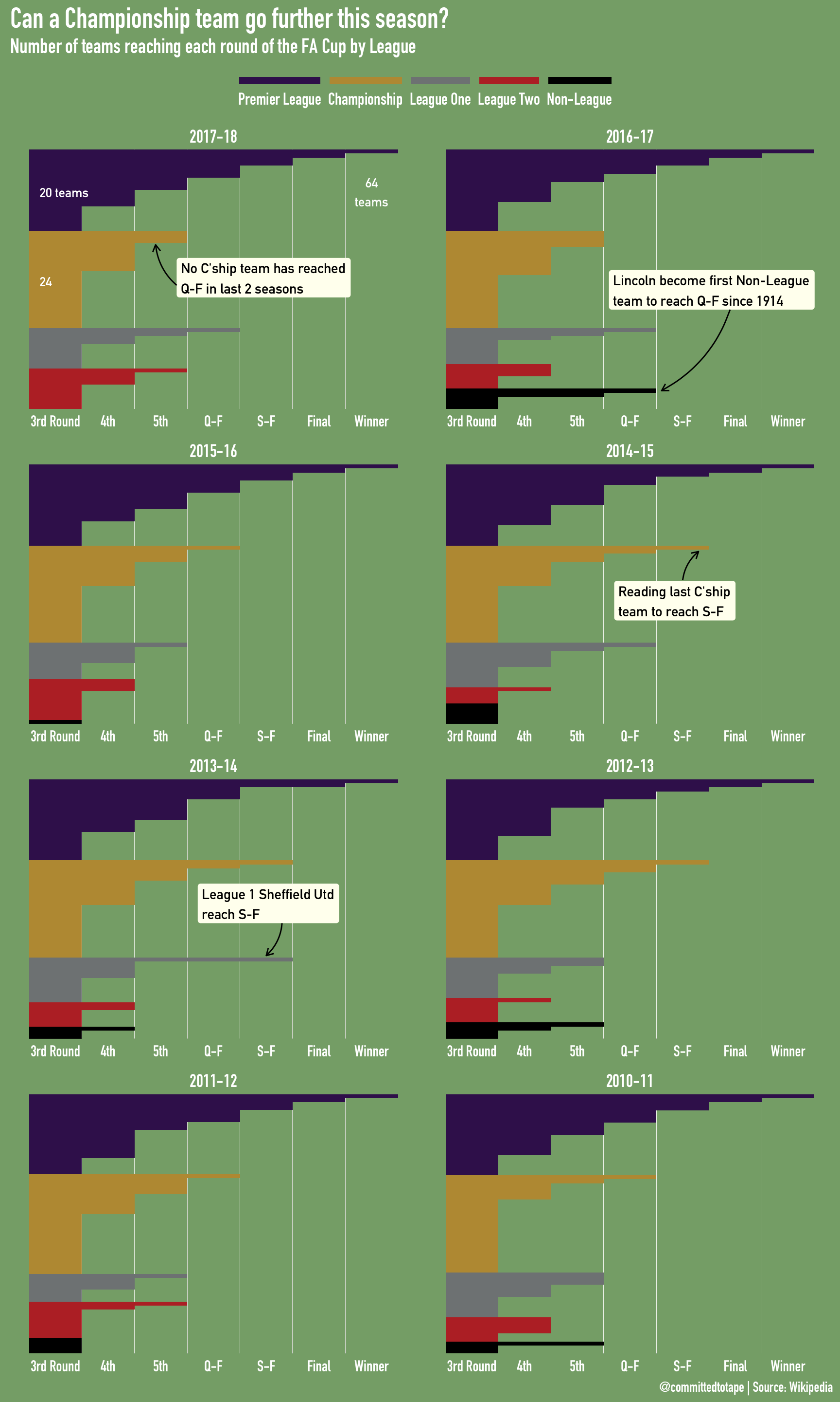
So, as I revealed at the top of this post, Championship teams have not made it passed the 5th round for the past 2 seasons, being surpassed by League One teams (and even Non-league Lincoln) in that period. The FA Cup final has been an all Premier League affair in the past 8 seasons, and 5 of the past 8 tournaments have seen Semi-finals contested by only Premier League teams.

Feedback Friday

I posted an original draft of this graphic on Twitter 3 weeks ago to get some feedback as part of a new initiative set up by JonTheGeek and the R4DS online learning community, called #RFeedbackFriday:

Just in time for #FACup weekend: Inspired by @FiveThirtyEight graph on Champions League (https://t.co/tB1xlh5hDn), I've done something similar for #FACup using #rstats with #rvest & #tidyverse #RFeedbackFriday pic.twitter.com/oLhGzDWwtH

— David Smale 🔎 (@committedtotape) January 25, 2019

After suggestions to add some more annotations and make them easier to read with a white-ish background, I updated the plot!

Using Twitter and the #Rstats community as a place to share and have people interact with my work has had a transformative affect on my development. As a solo learner it’s great to be connected (if only virtually) to a community where I can gain support and feedback, and further my skills. Thank you all, and maybe one day I will make it to the Third Round Proper!